Molecular Water solubility (LogS) prediction by Machine Learning Method
Posted onEdited on
Water solubility of compounds significantly affect its druggability, absorption and distribution property, such as oral bioavailability, intestinal absorption and BBB penetration. Typically, a low solubility goes along with a bad absorption and therefore the general aim is to avoid poorly soluble compounds. For convenient, water solubility (mol/Liter) are converted to logarithm value as LogS.
There are two major methods to predict LogS, atom contribution method and machine learning based method. The atom contribution method predict solubility via an increment system by adding atom contributions depending on their atom types. The machine learning method uses 2D or 3D features generated from molecular structures to fit a regression model for prediction.
The atom contribution method requires solid domain knowledge of cheminformatics, while machine learning method can use out-of-box cheminformatic toolkit to generate features for fitting models. Sounds easy, right? 😉
Here, we use python with rdkit and sklearn to predict LogS trained from a public dataset of water solubility
import os
import csv
import numpy as np
import pandas as pd
import matplotlib.pyplot as plt

from sklearn.externals import joblib
from sklearn.preprocessing import StandardScaler
from sklearn.model_selection import train_test_split
from sklearn.metrics import mean_absolute_error, r2_score, make_scorer

from rdkit import Chem
from rdkit.Chem import AllChem, DataStructs, Descriptors, ReducedGraphs
from rdkit.Avalon.pyAvalonTools import GetAvalonFP
from rdkit.ML.Descriptors import MoleculeDescriptors
from rdkit.Chem.EState import Fingerprinter
from rdkit.Chem import Descriptors

from sklearn.feature_selection import mutual_info_regression
defdescriptors(mol): calc=MoleculeDescriptors.MolecularDescriptorCalculator([x[0] for x in Descriptors._descList]) ds = np.asarray(calc.CalcDescriptors(mol)) return ds
Reading and Preprocessing
1
2
3
4
5
6
7
8
9
smis = [] logs = [] withopen("LogS.txt", "r") as f: reader = csv.reader(f, delimiter=" ") for row in reader: smis.append(row[1]) logs.append(float(row[2])) print(smis[:5], logs[:5])
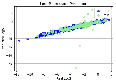
Train set R^2: 0.5843761663378015
Train MAE score: 0.7394
Test set R^2: 0.09632083916211343
Test MAE score: 1.4035
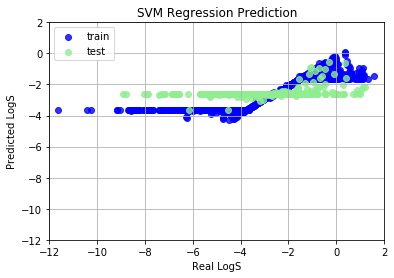
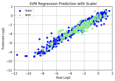
SVM Regression (SVR) model shows very bad prediction results, because we haven’t normalize features into (-1, 1). Data normalization can promote the performance in common machine learning problems, and speed up the coverage of gradient descent algorithm. We use StandardScaler, a rescaling method, to scale features to (-1, 1) range. After scaling, SVR works perfectly.
Train set R^2: 0.8662481382255657
Train MAE score: 0.5540
Test set R^2: 0.7600020560030265
Test MAE score: 0.7197
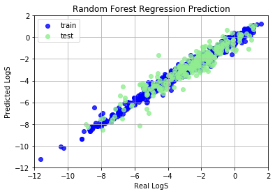
Random Forest Regression
Random Forest (RF) method is an ensemble method, which is an ensemble of Decision Tree models, thus we call it “Forest”. Feature normalization is not needed for RF, because RF didn’t compare magnitude of different features and it didn’t use gradient descent algorithm.
Train set R^2: 0.9826342744246852
Train MAE score: 0.1889
Test set R^2: 0.8906418060478993
Test MAE score: 0.4818
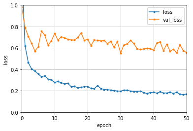
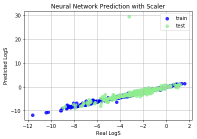
Neural Network Perception
Neural Network (NN) is a hot-topic after alpha-go defated the world champine, it can also used to build regression model. Here we will build a shallow NN to predict LogS
Train set R^2: 0.9901072859319796
Train MAE score: 0.1366
Test set R^2: -0.11753402040517735
Test MAE score: 0.5345
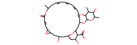
Obviously, NN predicted an abnormal value, why? Let’s dig out this abnormal compounds.
1 2 3 4 5 6 7 8 9
from rdkit.Chem.Draw import IPythonConsole v = X_test[np.argwhere(y_pred_test == y_pred_test.max())[0,0]] for smi, s inzip(smis, X): if np.all(s == v): abnorm_smi = smi print(abnorm_smi) m = Chem.MolFromSmiles(abnorm_smi) print(Descriptors.MolWt(m)) m
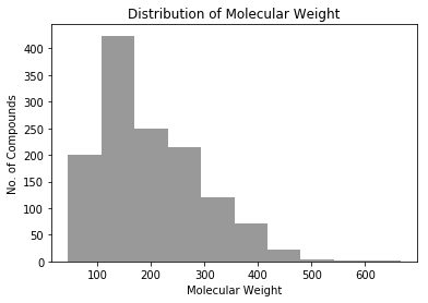
plt.xlabel("Molecular Weight") plt.ylabel("No. of Compounds") plt.title("Distribution of Molecular Weight") plt.hist(mws, color="gray", alpha=0.8) plt.show()
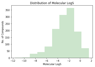
plt.xlabel("Molecular LogS") plt.ylabel("No. of Compounds") plt.title("Distribution of Molecular LogS") plt.hist(logs, color="green", alpha=0.2) plt.show()
This molecular is a macrocycle and has many hydrophilic functional groups. These hydrophilic groups contribute too much positive features and covered negative features of hydrophobic backbone. And of course, only 5 compounds have molecular weight greater than 500. Large compounds and macrocycles are unbalanced samples in this dataset, and this model is overfitted on small molecules.
This illustrate that it is not wise to predict LogS of large compounds and macrocycles by model trained on this dataset. On the other hand, this model is good at predicting LogS for small organic molecules.
Search for Best type of features
There are many kind of molecular finger prints and descriptors, which one or which kind of them is vital for LogS prediction?
# different features for fptype in ["MACCSKeys", "ErG", "Avalon", "ECFP", "Descriptor", "MACCSKeys+Descriptors"]: if fptype == "Descriptor": feature = [descriptors(mol) for mol in mols] elif fptype == "MACCSKeys+Descriptors": feature = [np.append(fingerprint(mol, "MACCSKeys"), descriptors(mol)) for mol in mols] else: feature = [fingerprint(mol, fptype) for mol in mols]
# random seed was set as 2 for reproduction np.random.seed(2) X = np.array(feature) y = np.array(logs)
model = SVR() model.fit(stds.transform(X_train), y_train) print("Feature Type:\t%s" % fptype) y_pred_train = model.predict(stds.transform(X_train)) print("\tTrain set R^2: ", r2_score(y_train, y_pred_train)) print("\tTrain MAE score: %.4f" % mean_absolute_error(y_train, y_pred_train))
y_pred_test = model.predict(stds.transform(X_test)) print("\tTest set R^2: ", r2_score(y_test, y_pred_test)) print("\tTest MAE score: %.4f" % mean_absolute_error(y_test, y_pred_test))
print("-"*40,"\n\n")
Feature Type: MACCSKeys
Train set R^2: 0.8348432537253556
Train MAE score: 0.5340
Test set R^2: 0.7269931078788134
Test MAE score: 0.7887
----------------------------------------
Feature Type: ErG
Train set R^2: 0.43533956678068464
Train MAE score: 1.0801
Test set R^2: 0.41443974442003917
Test MAE score: 1.1513
----------------------------------------
Feature Type: Avalon
Train set R^2: 0.8411296883499888
Train MAE score: 0.5065
Test set R^2: 0.7501108238770297
Test MAE score: 0.7341
----------------------------------------
Feature Type: ECFP
Train set R^2: 0.7829458742941775
Train MAE score: 0.5726
Test set R^2: 0.5447519853586031
Test MAE score: 1.0134
----------------------------------------
Feature Type: Descriptor
Train set R^2: 0.9429008343024807
Train MAE score: 0.3142
Test set R^2: 0.892167479543334
Test MAE score: 0.4646
----------------------------------------
Feature Type: MACCSKeys+Descriptors
Train set R^2: 0.9529119367162064
Train MAE score: 0.2789
Test set R^2: 0.8969447643834331
Test MAE score: 0.4498
----------------------------------------
1 2 3 4 5 6 7 8 9 10 11 12 13 14 15 16 17 18
# different feature selection cutoff minfo = mutual_info_regression(X_train, y_train) for cutoff in (0., 0.01, 0.05, 0.1): print("Feature left at cutoff %.2f:\t%d feature" % (cutoff, np.sum(minfo > cutoff))) stds = StandardScaler() stds.fit(X_train[:, minfo > cutoff])
model = SVR() model.fit(stds.transform(X_train[:, minfo > cutoff]), y_train)
y_pred_train = model.predict(stds.transform(X_train[:, minfo > cutoff])) print("\tTrain set R^2: ", r2_score(y_train, y_pred_train)) print("\tTrain MAE score: %.4f" % mean_absolute_error(y_train, y_pred_train))
Feature left at cutoff 0.00:	300 feature
	Train set R^2:  0.9547396313014773
	Train MAE score: 0.2688
	Test set R^2:  0.9018933828417203
	Test MAE score: 0.4386
----------------------------------------


Feature left at cutoff 0.01:	232 feature
	Train set R^2:  0.9560197972695562
	Train MAE score: 0.2641
	Test set R^2:  0.9144409662106348
	Test MAE score: 0.4106
----------------------------------------


Feature left at cutoff 0.05:	107 feature
	Train set R^2:  0.9388813570437281
	Train MAE score: 0.3228
	Test set R^2:  0.905214588528981
	Test MAE score: 0.4471
----------------------------------------


Feature left at cutoff 0.10:	73 feature
	Train set R^2:  0.9306199986641003
	Train MAE score: 0.3609
	Test set R^2:  0.8990763861247755
	Test MAE score: 0.4719
----------------------------------------
Conclusion
In this article, I used different models, features and feature selection cutoff to build a state-of-art LogS prediction model on a public dataset. On this dataset, my SVR-0.01 model (R^2 0.92, MAE:0.41) shows best performance on test set. Roughly compared to other blog and ALOGPS, this model shows best performance, but I still need an external validation set to estimate its generalization. Since most compounds in this dataset are soluble (-8 < LogS < 2) small compounds (50 < MW < 400), this model is very suitable to estimate drug-like moleculars LogS.